
To recap, usched is an experimental (and very simple, 120LOC) coroutine implementation different from stackful and stackless models: coroutines are executed on the native stack of the caller and when the coroutine is about to block its stack is copied into a separately allocated (e.g., in the heap) buffer. The buffer is copied back onto the native stack when the coroutine is ready to resume.
I added a new scheduler ll.c that distributes coroutines across multiple native threads and then does lockless scheduling within each thread. In the benchmark (the same as in the previous post), each coroutine in the communicating cycle belongs to the same thread.
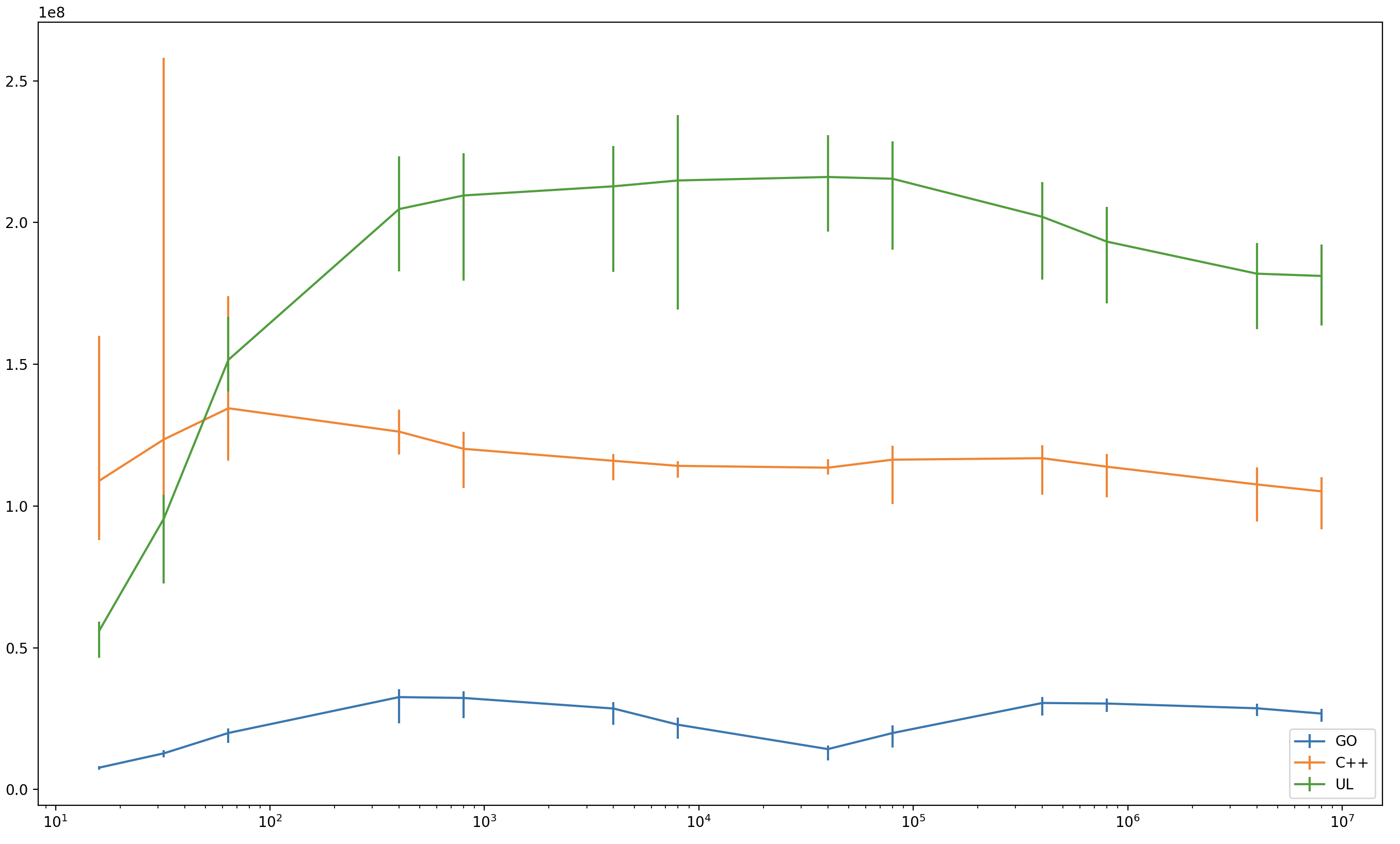
Results are amazing: usched actually beats compiler-assisted C++ coroutines by a large margin. The horizontal axis is the number of coroutines in the test (logarithmic) and the vertical axis is coroutine wakeup-wait operations per second (1 == 1e8 op/sec).
| 16 | 32 | 64 | 400 | 800 | 4000 | 8000 | 40000 | 80000 | 400000 | 800000 | 4M | 8M | |
|---|---|---|---|---|---|---|---|---|---|---|---|---|---|
| GO | 0.077 | 0.127 | 0.199 | 0.326 | 0.323 | 0.285 | 0.228 | 0.142 | 0.199 | 0.305 | 0.303 | 0.286 | 0.268 |
| C++ | 1.089 | 1.234 | 1.344 | 1.262 | 1.201 | 1.159 | 1.141 | 1.135 | 1.163 | 1.168 | 1.138 | 1.076 | 1.051 |
| UL | 0.560 | 0.955 | 1.515 | 2.047 | 2.095 | 2.127 | 2.148 | 2.160 | 2.154 | 2.020 | 1.932 | 1.819 | 1.811 |
I only kept the most efficient implementation from every competing class: C++ for stackless, GO for stackful and usched for stackswap. See the full results in results.darwin
#include <memory>
#include <string>
#include <cassert>
#include <iostream>
#include <coroutine>
#include <cppcoro/generator.hpp>

struct tnode;
using tree = std::shared_ptr<tnode>;
struct tnode {
	tree left;
	tree right;
	tnode() {};
	tnode(tree l, tree r) : left(l), right(r) {}
};

auto print(tree t) -> std::string {
	return  t ? (std::string{"["} + print(t->left) + " "
		     + print(t->right) + "]") : "*";
}

cppcoro::generator<tree> gen(int n) {
	if (n == 0) {
		co_yield nullptr;
	} else {
		for (int i = 0; i < n; ++i) {
			for (auto left : gen(i)) {
				for (auto right : gen(n - i - 1)) {
					co_yield tree(new tnode(left, right));
				}
			}
		}
	}
}

int main(int argc, char **argv) {
	for (auto t : gen(std::atoi(argv[1]))) {
		std::cout << print(t) << std::endl;
	}
}
$ for i in $(seq 0 1000000) ;do ./gen $i | wc -l ;done
       1
       1
       2
       5
      14
      42
     132
     429
    1430
    4862
   16796
   58786
  208012
  742900
This repository (https://github.com/nikitadanilov/usched) contains a simple experimental implementation of coroutines alternative to well-known "stackless" and "stackful" methods.
The term "coroutine" gradually grew to mean a mechanism where a computation, which in this context means a chain of nested function calls, can "block" or "yield" so that the top-most caller can proceed and the computation can later be resumed at the blocking point with the chain of intermediate function activation frames preserved.
Prototypical uses of coroutines are lightweight support for potentially blocking operations (user interaction, IO, networking) and generators, which produce multiple values (see same fringe problem).
There are two common coroutine implementation methods:
a stackful coroutine runs on a separate stack. When a stackful coroutine blocks, it performs a usual context switch. Historically "coroutines" meant stackful coroutines. Stackful coroutines are basically little more than usual threads, and so they can be kernel (supported by the operating system) or user-space (implemented by a user-space library, also known as green threads), preemptive or cooperative.
a stackless coroutine does not use any stack when blocked. In a typical implementation instead of using a normal function activation frame on the stack, the coroutine uses a special activation frame allocated in the heap so that it can outlive its caller. Using heap-allocated frame to store all local variable lends itself naturally to compiler support, but some people are known to implement stackless coroutines manually via a combination of pre-processing, library and tricks much worse than Duff's device.
Stackful and stateless are by no means the only possibilities. One of the earliest languages to feature generators CLU (distribution) ran generators on the caller's stack.
usched is in some sense intermediate between stackful and stackless: its coroutines do not use stack when blocked, nor do they allocate individual activation frames in the heap.
The following is copied with some abbreviations from usched.c.
usched: A simple dispatcher for cooperative user-space threads.
A typical implementation of user-space threads allocates a separate stack for
each thread when the thread is created and then dispatches threads (as
decided by the scheduler) through some context switching mechanism, for
example, longjmp().
In usched all threads (represented by struct ustack) are executed on the same
"native" stack. When a thread is about to block (usched_block()), a memory
buffer for the stack used by this thread is allocated and the stack is copied
to the buffer. After that the part of the stack used by the blocking thread
is discarded (by longjmp()-ing to the base of the stack) and a new thread is
selected. The stack of the selected thread is restored from its buffer and
the thread is resumed by longjmp()-ing to the usched_block() that blocked it.
The focus of this implementation is simplicity: the total size of usched.[ch]
is less than 120LOC, as measured by SLOCCount.
Advantages:
no need to allocate maximal possible stack at thread initialisation: stack buffer is allocated as needed. It is also possible to free the buffer when the thread is resumed (not currently implemented);
thread that doesn't block has 0 overhead: it is executed as a native function call (through a function pointer) without any context switching;
because the threads are executed on the stack of the same native underlying thread, native synchronisation primitives (mutices, etc.) work, although the threads share underlying TLS. Of course one cannot use native primitives to synchronise between usched threads running on the same native thread.
Disadvantages:
stack copying introduces overhead (memcpy()) in each context switch;
because stacks are moved around, addresses on a thread stack are only valid while the thread is running. This invalidates certain common programming idioms: other threads and heap cannot store pointers to the stacks, at least to the stacks of the blocked threads. Note that Go language, and probably other run-times, maintains a similar invariant.
usched is only a dispatcher and not a scheduler: it blocks and resumes threads but
it does not keep track of threads (specifically allocation and freeing of struct ustack instances is done elsewhere),
it implements no scheduling policies.
These things are left to the user, together with stack buffers allocation and freeing. The user supplies 3 call-backs:
usched::s_next(): the scheduling function. This call-backs returns the next
thread to execute. This can be either a new (never before executed) thread
initialised with ustack_init(), or it can be a blocked thread. The user must
keep track of blocked and runnable threads, presumably by providing wrappers
to ustack_init() and ustack_block() that would record thread state changes. It
is up to usched::s_next() to block and wait for events if there are no
runnable threads and all threads are waiting for something;
usched::s_alloc(): allocates new stack buffer of at least the specified
size. The user have full control over stack buffer allocation. It is possible
to pre-allocate the buffer when the thread is initialised (reducing the cost
of usched_block()), it is possible to cache buffers, etc.;
usched::s_free(): frees the previously allocated stack buffer.
rr.h and rr.c provide a simple "round-robin" scheduler implementing all the call-backs. Use it carefully, it was only tested with rmain.c benchmark.
The following diagrams show stack management by usched. The stack grows from right to left.
At the entrance to the dispatcher loop. usched_run(S):
usched_run()
A new (never before executed) thread U is selected by S->s_next(), launch()
calls the thread startup function U->u_f():
U->u_f() launch() usched_run()
The thread executes as usual on the stack, until it blocks by calling
usched_block():
usched_block() bar() U->u_f() launch() usched_run()
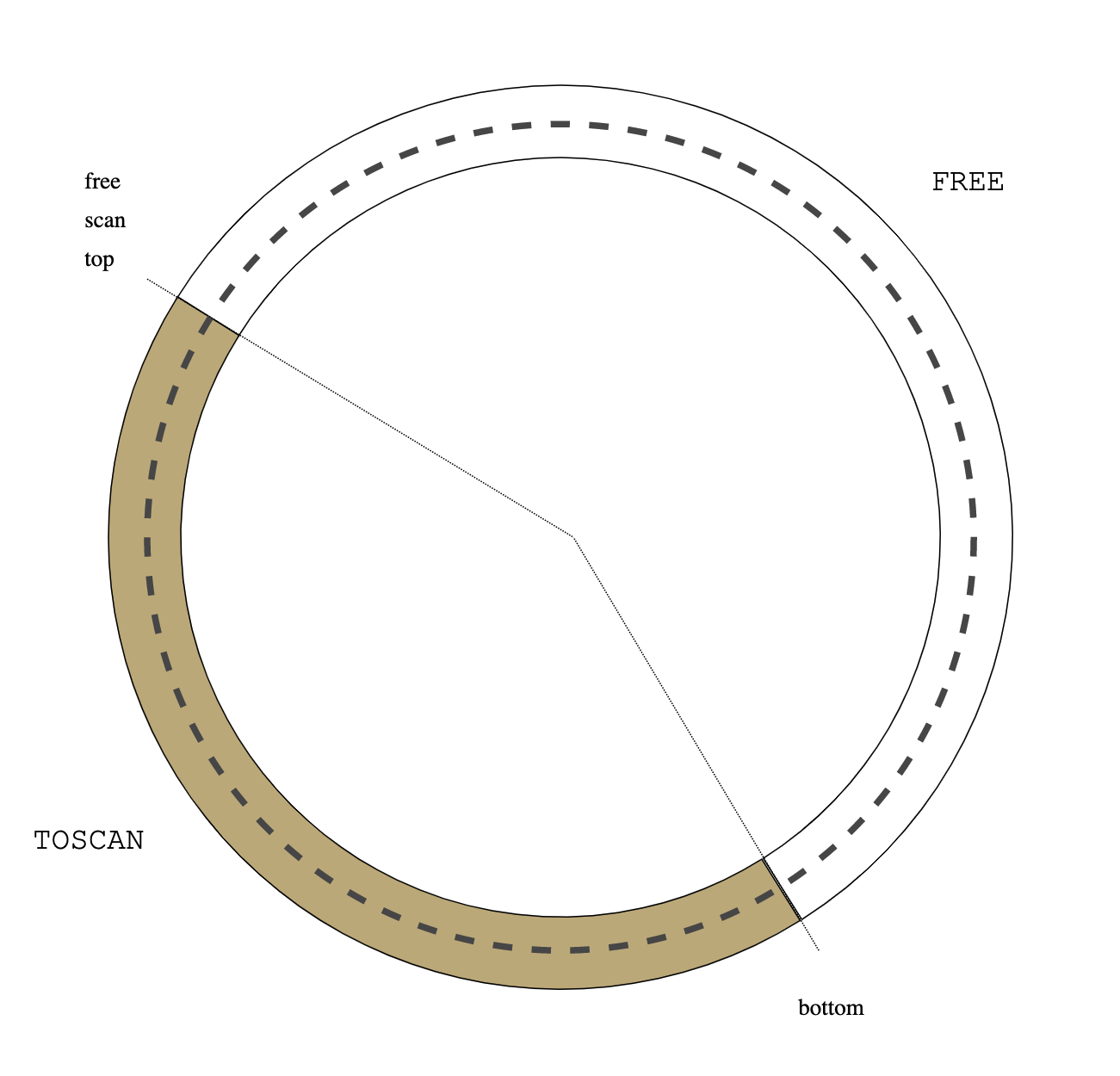
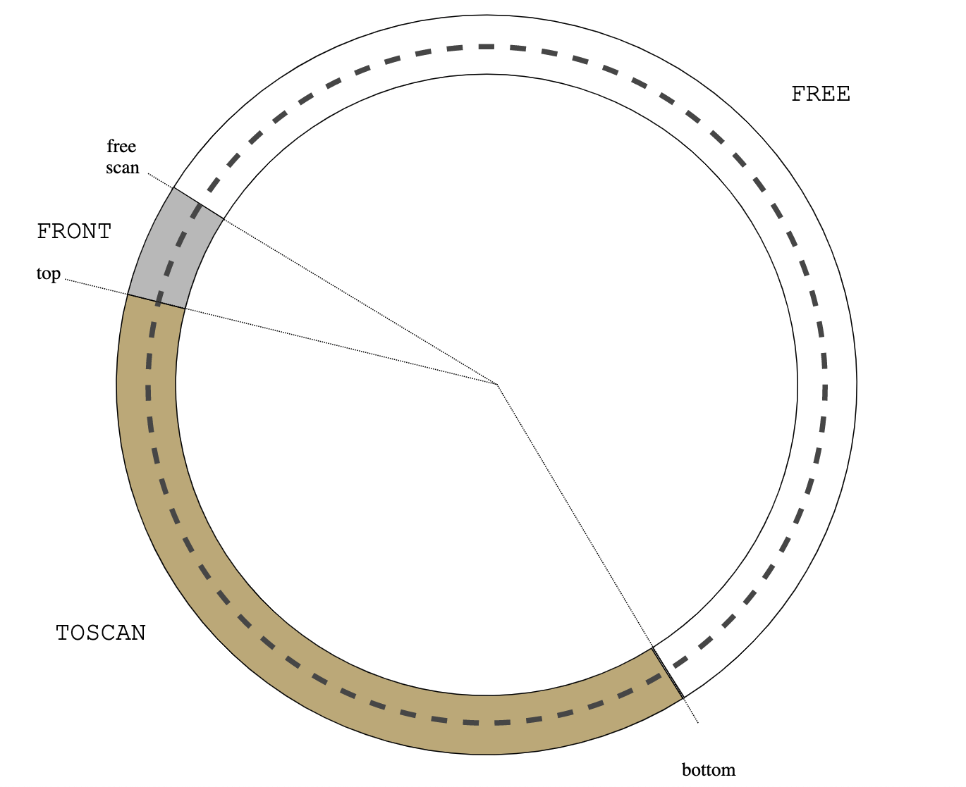
The stack from U->u_top to U->u_bottom is copied into the stack buffer
U->u_stack, and control returns to usched_run() by longjmp(S->s_buf):
usched_run()
Next, suppose S->s_next() selects a previously blocked thread V ready to be
resumed. usched_run() calls cont(V).
cont() usched_run()
cont() copies the stack from the buffer to [V->u_top, V->u_bottom]
range. It's important that this memcpy() operation does not overwrite
cont()'s own stack frame, this is why pad[] array is needed in launch(): it
advances V->u_bottom and gives cont() some space to operate.
usched_block() foo() V->u_f() cont() usched_run()
Then cont() longjmp()-s to V->u_cont, restoring V execution context:
usched_block() foo() V->u_f() cont() usched_run()
V continues its execution as if it returned from usched_block().
By design, a single instance of struct usched cannot take advantage of
multiple processors, because all its threads are executing within a single
native thread. Multiple instances of struct usched can co-exist within a
single process address space, but a ustack thread created for one instance
cannot be migrated to another. One possible strategy to add support for multiple
processors is to create multiple instances of struct usched and schedule them
(that is, schedule the threads running respective usched_run()-s) to
processors via pthread_setaffinity_np() or similar. See
rr.c for a
simplistic implementation.
the stack is assumed to grow toward lower addresses. This is easy to fix, if necessary;
the implementation is not signal-safe. Fixing this can be as easy as replacing *jmp() calls with their sig*jmp() counterparts. At the moment signal-based code, like gperf -lprofiler library, would most likely crash usched;
usched.c must be compiled without optimisations and with
-fno-stack-protector option (gcc);
usched threads are cooperative: a thread will continue to run until it
completes of blocks. Adding preemption (via signal-based timers) is
relatively easy, the actual preemption decision will be relegated to the
external "scheduler" via a new usched::s_preempt() call-back invoked from
a signal handler.
Midori seems to use a similar method: a coroutine (called activity there) starts on the native stack. If it needs to block, frames are allocated in the heap (this requires compiler support) and filled in from the stack, the coroutine runs in these heap-allocated frames when resumed.
usched was benchmarked against a few stackful (go, pthreads) and stackless (rust, c++ coroutines) implementations. A couple of caveats:
all benchmarking in general is subject to the reservations voiced by Hippocrates and usually translated (with the complete reversal of the meaning) as ars longa, vita brevis, which means: "the art [of doctor or tester] takes long time to learn, but the life of a student is brief, symptoms are vague, chances of success are doubtful".
the author is much less than fluent with all the languages and frameworks used in the benchmarking. It is possible that some of the benchmarking code is inefficient or just outright wrong. Any comments are appreciated.
The benchmark tries to measure the efficiency of coroutine switching. It creates R cycles, N coroutines each. Each cycle performs M rounds, where each round consists of sending a message across the cycle: a particular coroutine (selected depending on the round number) sends the message to its right neighbour, all other coroutines relay the message received from the left to the right, the round completes when the originator receives the message after it passed through the entire cycle.
If N == 2, the benchmark is R pairs of processes, ping-ponging M messages within each pair.
Some benchmarks support two additional parameters: D (additional space in bytes, artificially consumed by each coroutine in its frame) and P (the number of native threads used to schedule the coroutines.
The benchmark creates N*R coroutines and sends a total of N*R*M messages, the latter being proportional to the number of coroutine switches.
bench.sh runs all implementations with the same N, R and M parameters. graph.py plots the results.
POSIX. Source: pmain.c, binary: pmain. Pthreads-based stackful implementation in C. Uses default thread attributes. pmain.c also contains emulation of unnamed POSIX semaphores for Darwin. Plot label: "P". This benchmarks crashes with "pmain: pthread_create: Resource temporarily unavailable" for large values of N*R.
Go. Source: gmain.go, binary: gmain. The code is straightforward (it was a pleasure to write). D is supported via runtime.GOMAXPROCS(). "GO1T" are the results for a single native thread, "GO" are the results without the restriction on the number of threads.
Rust. Source: cycle/src/main.rs, binary: cycle/target/release/cycle. Stackless implementation using Rust builtin async/.await. Label: "R". It is single-threaded (I haven't figured out how to distribute coroutines to multiple executors), so should be compared with GO1T, C++1T and U1T. Instead of fighting with the Rust borrow checker, I used "unsafe" and shared data-structures between multiple coroutines much like other benchmarks do.
C++. Source:
c++main.cpp,
binary: c++main. The current state of coroutine support in C++ is unclear. Is
everybody supposed to directly use <coroutine> interfaces or one of the
mutually incompatible libraries that provide easier to use interfaces on top
of <coroutine>? This benchmark uses Lewis
Baker's
cppcoro, (Andreas
Buhr's
fork). Labels: "C++" and "C++1T" (for
single-threaded results).
usched. Source:
rmain.c,
binary: rmain. Based on usched.[ch] and rr.[ch] This is our main interest,
so we test a few combinations of parameters.
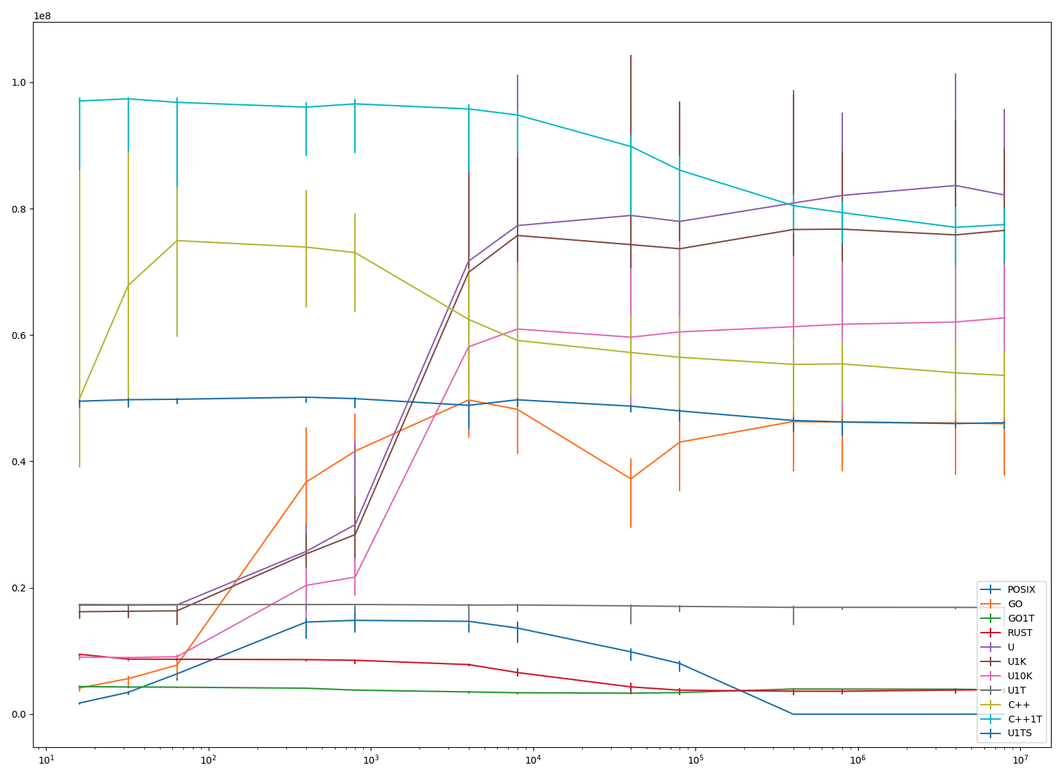
-DSINGLE_THREAD compilation option, a separate binary rmain.1t).bench.sh runs all benchmarks with N == 2 (message ping-pong) and N == 8. Raw results are in results.linux. In the graphs, the horizontal axis is the number of coroutines (N*R, logarithmic) and the vertical axis is the operations (N*R*M) per second
Environment: Linux VM, 16 processors, 16GB of memory. Kernel: 4.18.0 (Rocky Linux).
| 16 | 32 | 64 | 400 | 800 | 4000 | 8000 | 40000 | 80000 | 400000 | 800000 | 4000000 | 8000000 | |
|---|---|---|---|---|---|---|---|---|---|---|---|---|---|
| POSIX | 1.76 | 3.46 | 6.39 | 14.58 | 14.85 | 14.70 | 13.63 | 9.87 | 8.02 | 0.00 | 0.00 | 0.00 | 0.01 |
| GO | 4.14 | 5.62 | 7.77 | 36.74 | 41.64 | 49.72 | 48.24 | 37.24 | 43.06 | 46.31 | 46.22 | 46.09 | 45.95 |
| GO1T | 4.38 | 4.30 | 4.27 | 4.11 | 3.81 | 3.53 | 3.40 | 3.33 | 3.43 | 3.99 | 3.98 | 3.95 | 3.86 |
| RUST | 9.48 | 8.71 | 8.69 | 8.64 | 8.53 | 7.85 | 6.59 | 4.32 | 3.80 | 3.63 | 3.63 | 3.83 | 3.90 |
| U | 17.24 | 17.27 | 17.30 | 25.77 | 29.99 | 71.68 | 77.32 | 78.92 | 77.98 | 80.88 | 82.09 | 83.66 | 82.15 |
| U1K | 16.21 | 16.29 | 16.35 | 25.38 | 28.41 | 69.92 | 75.76 | 74.31 | 73.65 | 76.69 | 76.75 | 75.84 | 76.56 |
| U10K | 9.04 | 8.96 | 9.09 | 20.38 | 21.69 | 58.13 | 60.95 | 59.66 | 60.50 | 61.32 | 61.71 | 62.06 | 62.72 |
| U1T | 17.37 | 17.31 | 17.35 | 17.35 | 17.36 | 17.27 | 17.29 | 17.14 | 17.06 | 16.91 | 16.91 | 16.91 | 16.87 |
| C++ | 49.87 | 67.85 | 74.94 | 73.91 | 73.04 | 62.48 | 59.15 | 57.23 | 56.48 | 55.35 | 55.44 | 54.02 | 53.61 |
| C++1T | 97.03 | 97.38 | 96.82 | 96.06 | 96.58 | 95.78 | 94.83 | 89.83 | 86.09 | 80.48 | 79.37 | 77.04 | 77.48 |
| U1TS | 49.53 | 49.76 | 49.83 | 50.16 | 49.93 | 48.88 | 49.75 | 48.75 | 47.99 | 46.48 | 46.25 | 45.99 | 46.12 |
| UL | 76.03 | 116.63 | 160.72 | 169.74 | 169.99 | 171.57 | 170.32 | 165.82 | 169.43 | 174.32 | 171.55 | 169.48 | 170.04 |
(N == 8) A few notes:
As mentioned above, pthreads-based solution crashes with around 50K threads.
Most single-threaded versions ("GO1T", "R" and "U1T") are stable as corpse's body temperature. Rust cools off completely at about 500K coroutines. Single-threaded C++ ("C++1T") on the other hand is the most performant solution for almost the entire range of measurement, it is only for coroutine counts higher than 500K when "U" overtakes it.
It is interesting that a very simple and unoptimised usched fares so well against heavily optimized C++ and Go run-times. (Again, see the reservations about the benchmarking.)
Rust is disappointing: one would hope to get better results from a rich type combined with compiler support.
| 4 | 8 | 16 | 100 | 200 | 1000 | 2000 | 10000 | 20000 | 100000 | 200000 | 1000000 | 2000000 | |
|---|---|---|---|---|---|---|---|---|---|---|---|---|---|
| POSIX | 0.56 | 0.97 | 1.84 | 6.36 | 6.88 | 7.78 | 7.82 | 7.58 | 7.15 | 5.34 | 0.00 | 0.00 | 0.00 |
| GO | 7.40 | 11.03 | 19.23 | 40.44 | 45.79 | 51.81 | 52.87 | 52.77 | 53.15 | 53.62 | 53.22 | 55.77 | 56.82 |
| GO1T | 4.54 | 4.55 | 4.53 | 4.53 | 4.53 | 4.52 | 4.52 | 4.50 | 4.47 | 4.36 | 4.31 | 4.26 | 4.26 |
| RUST | 5.68 | 5.75 | 5.75 | 4.74 | 4.74 | 4.62 | 4.46 | 4.13 | 3.70 | 2.81 | 2.77 | 2.76 | 2.73 |
| U | 11.22 | 11.27 | 11.26 | 11.30 | 7.91 | 24.66 | 38.72 | 35.67 | 40.60 | 41.18 | 42.06 | 42.96 | 42.74 |
| U1K | 9.64 | 9.62 | 9.65 | 9.67 | 7.61 | 22.14 | 34.38 | 31.70 | 34.54 | 34.56 | 34.59 | 35.47 | 35.56 |
| U10K | 4.43 | 4.62 | 4.50 | 4.25 | 5.02 | 15.79 | 26.18 | 25.33 | 27.60 | 27.62 | 27.63 | 27.72 | 28.16 |
| U1T | 11.24 | 11.29 | 11.34 | 11.26 | 11.32 | 11.30 | 11.28 | 11.28 | 11.22 | 11.19 | 11.15 | 11.13 | 11.15 |
| C++ | 46.33 | 46.30 | 63.38 | 114.30 | 117.05 | 114.12 | 111.36 | 101.32 | 100.13 | 84.30 | 78.53 | 72.77 | 71.00 |
| C++1T | 96.56 | 96.03 | 96.37 | 95.97 | 95.49 | 95.68 | 94.94 | 92.95 | 91.23 | 83.55 | 80.33 | 77.22 | 76.22 |
| U1TS | 19.59 | 19.66 | 19.80 | 19.87 | 19.89 | 19.86 | 19.82 | 19.72 | 19.66 | 19.51 | 19.45 | 19.33 | 19.37 |
| UL | 12.19 | 23.48 | 50.39 | 65.71 | 67.22 | 69.17 | 70.01 | 70.09 | 69.36 | 69.28 | 69.43 | 68.83 | 68.00 |
(N == 2)
First, note that the scale is different on the vertical axis.
Single-threaded benchmarks display roughly the same behaviour (exactly the same in "C++1T" case) as with N == 8.
Go is somewhat better. Perhaps its scheduler is optimised for message ping-pong usual in channel-based concurrency models?
usched variants are much worse (50% worse for "U") than N == 8.
Rust is disappointing.
To reproduce:
$ # install libraries and everything, then...
Overall, the results are surprisingly good. The difference between "U1T" and "U1TS" indicates that the locking in rr.c affects performance significantly, and affects it even more with multiple native threads, when locks are contended across processors. I'll try to produce a more efficient (perhaps lockless) version of a scheduler as the next step.
3-lisp is a dialect of Lisp designed and implemented by Brian C. Smith as part of his PhD. thesis Procedural Reflection in Programming Languages (what this thesis refers to as "reflection" is nowadays more usually called "reification"). A 3-lisp program is conceptually executed by an interpreter written in 3-lisp that is itself executed by an interpreter written in 3-lisp and so on ad infinitum. This forms a (countably) infinite tower of meta-circular (v.i.) interpreters. reflective lambda is a function that is executed one tower level above its caller. Reflective lambdas provide a very general language extension mechanism.
The code is here.An interpreter is a program that executes programs written in some programming language.
A meta-circular interpreter is an interpreter for a programming language written in that language. Meta-circular interpreters can be used to clarify or define the semantics of the language by reducing the full language to a sub-language in which the interpreter is expressed. Historically, such definitional interpreters become popular within the functional programming community, see the classical Definitional interpreters for higher-order programming languages. Certain important techniques were classified and studied in the framework of meta-circular interpretation, for example, continuation passing style can be understood as a mechanism that makes meta-circular interpretation independent of the evaluation strategy: it allows an eager meta-language to interpret a lazy object language and vice versa. As a by-product, a continuation passing style interpreter is essentially a state machine and so can be implemented in hardware, see The Scheme-79 chip. Similarly, de-functionalisation of languages with higher-order functions obtains for them first-order interpreters. But meta-circular interpreters occur in imperative contexts too, for example, the usual proof of the Böhm–Jacopini theorem (interestingly, it was Corrado Böhm who first introduced meta-circular interpreters in his 1954 PhD. thesis) constructs for an Algol-like language a meta-circular interpreter expressed in some goto-less subset of the language and then specialises this interpreter for a particular program in the source language.
Given a language with a meta-circular interpreter, suppose that the language is extended with a mechanism to trap to the meta-level. For example, in a lisp-like language, that trap can be a new special form (reflect FORM) that directly executes (rather than interprets) FORM within the interpreter. Smith is mostly interested in reflective (i.e., reification) powers obtained this way, and it is clear that the meta-level trap provides a very general language extension method: one can add new primitives, data types, flow and sequencing control operators, etc. But if you try to add reflect to an existing LISP meta-circular interpreter (for example, see p. 13 of LISP 1.5 Programmers Manual) you'd hit a problem: FORM cannot be executed at the meta-level, because at this level it is not a form, but an S-expression.
To understand the nature of the problem, consider a very simple case: the object language is the machine language (or equivalently the assembly language) of some processor. Suppose that the interpreter for the machine code is written in (or, more realistically, compiled to) the same machine language. The interpreter maintains the state of the simulated processor that is, among other things registers and memory. Say, the object (interpreted) code can access a register, R0, then the interpreter has to keep the contents of this register somewhere, but typically not in its (interpreter's) R0. Similarly, a memory word visible to the interpreted code at an address ADDR is stored by the interpreter at some, generally different, address ADDR' (although, by applying the contractive mapping theorem and a lot of hand-waving one might argue that there will be at least one word stored at the same address at the object- and meta-levels). Suppose that the interpreted machine language has the usual sub-routine call-return instructions call ADDR and return and is extended with a new instruction reflect ADDR that forces the interpreter to call the sub-routine ADDR. At the very least the interpreter needs to convert ADDR to the matching ADDR'. This might not be enough because, for example, the object-level sub-routine ADDR might not be contiguous at the meta-level, i.e., it is not guaranteed that if ADDR maps to ADDR' then (ADDR + 1) maps (ADDR' + 1). This example demonstrates that a reflective interpreter needs a systematic and efficient way of converting or translating between object- and meta-level representations. If such a method is somehow provided, reflect is a very powerful mechanism: by modifying interpreter state and code it can add new instructions, addressing modes, condition bits, branch predictors, etc.
In his thesis Prof. Smith analyses what would it take to construct a dialect of LISP for which a faithful reflective meta-circular interpreter is possible. He starts by defining a formal model of computation with an (extremely) rigorous distinction between meta- and object- levels (and, hence, between use and mention). It is then determined that this model can not be satisfactorily applied to the traditional LISP (which is called 1-LISP in the thesis and is mostly based on Maclisp). The reason is that LISP's notion of evaluation conflates two operations: normalisation that operates within the level and reference that moves one level down. A dialect of LISP that consistently separates normalisation and reference is called 2-LISP (the then new Scheme is called LISP-1.75). Definition of 2-LISP occupies the bulk of the thesis, which the curious reader should consult for (exciting, believe me) details.
Once 2-LISP is constructed, adding the reflective capability to it is relatively straightforward. Meta-level trap takes the form of a special lambda expression:
(lambda reflect [ARGS ENV CONT] BODY)When this lambda function is applied (at the object level), the body is directly executed (not interpreted) at the meta-level with ARGS bound to the meta-level representation of the actual parameters, ENV bound to the environment (basically, the list of identifiers and the values they are bound to) and CONT bound to the continuation. Environment and continuation together represent the 3-LISP interpreter state (much like registers and memory represent the machine language interpreter state), this representation goes all the way back to SECD machine, see The Mechanical Evaluation of Expressions.
Here is the fragment of 3-LISP meta-circular interpreter code that handles lambda reflect (together with "ordinary" lambda-s, denoted by lambda simple):
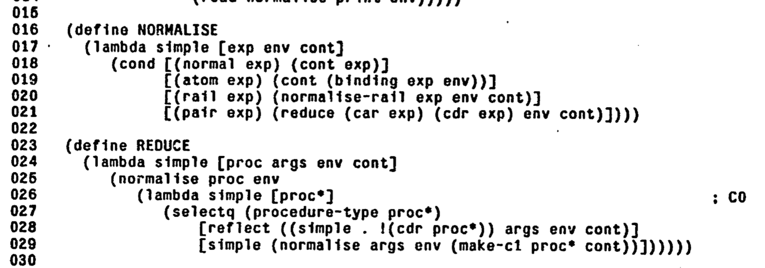
It is of course not possible to run an infinite tower of interpreters directly.
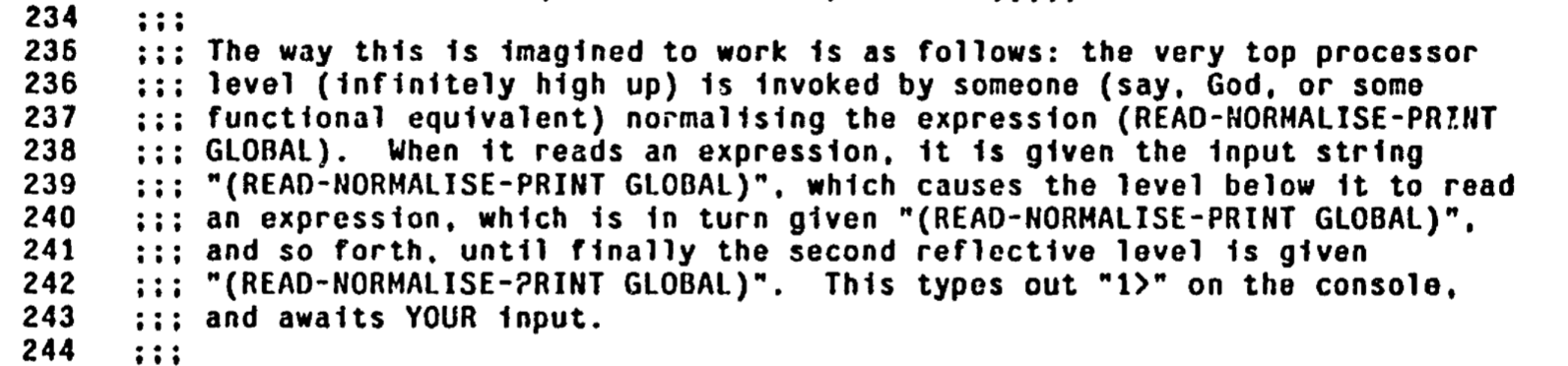
3-LISP implementation creates a meta-level on demand, when a reflective lambda is invoked. At that moment the state of the meta-level interpreter is synthesised (e.g., see make-c1 in the listing above). The implementation takes pain to detect when it can drop down to a lower level, which is not entirely simple because a reflective lambda can, instead of returning (that is, invoking the supplied continuation), run a potentially modified version of the read-eval-loop (called READ-NORMALISE-PRINT (see) in 3-LISP) which does not return. There is a lot of non-trivial machinery operating behind the scenes and though the implementation modestly proclaims itself EXTREMELY INEFFICIENT it is, in fact, remarkably fast.
I was unable to find a digital copy of the 3-LISP sources and so manually retyped the sources from the appendix of the thesis. The transcription in 3-lisp.lisp (2003 lines, 200K characters) preserves the original pagination and character set, see the comments at the top of the file. Transcription was mostly straightforward except for a few places where the PDF is illegible (for example, here) all of which fortunately are within comment blocks.
The sources are in CADR machine dialect of LISP, which, save for some minimal and no longer relevant details, is equivalent to Maclisp.
3-LISP implementation does not have its own parser or interpreter. Instead, it uses flexibility built in a lisp reader (see, readtables) to parse, interpret and even compile 3-LISP with a very small amount of additional code. Amazingly, this more than 40 years old code, which uses arcane features like readtable customisation, runs on a modern Common Lisp platform after a very small set of changes: some functions got renamed (CASEQ to CASE, *CATCH to CATCH, etc.), some functions are missing (MEMQ, FIXP), some signatures changed (TYPEP, BREAK, IF). See 3-lisp.cl for details.
Unfortunately, the port does not run on all modern Common Lisp implementations, because it relies on the proper support for backquotes across recursive reader invocations:
;;     Maclisp maintains backquote context across recursive parser;;     invocations. For example in the expression (which happens within defun
;;     3-EXPAND-PAIR)
;;
;;         `\(PCONS ~,a ~,d)
;;
;;     the backquote is consumed by the top-level activation of READ. Backslash
;;     forces the switch to 3-lisp readtable and call to 3-READ to handle the
;;     rest of the expression. Within this 3-READ activation, the tilde forces
;;     switch back to L=READTABLE and a call to READ to handle ",a". In Maclisp,
;;     this second READ activation re-uses the backquote context established by
;;     the top-level READ activation. Of all Common Lisp implementations that I
;;     tried, only sbcl correctly handles this situation. Lisp Works and clisp
;;     complain about "comma outside of backquote". In clisp,
;;     clisp-2.49/src/io.d:read_top() explicitly binds BACKQUOTE-LEVEL to nil.
Among Common Lisp implementations I tried, only sbcl supports it properly. After reading Common Lisp Hyperspec, I believe that it is Maclisp and sbcl that implement the specification correctly and other implementations are faulty.
Procedural Reflection in Programming Languages is, in spite of its age, a very interesting read. Not only does it contain an implementation of a refreshingly new and bold idea (it is not even immediately obvious that infinite reflective towers can at all be implemented, not to say with any reasonable degree of efficiency), it is based on an interplay between mathematics and programming: the model of computation is proposed and afterward implemented in 3-LISP. Because the model is implemented in an actual running program, it has to be specified with extreme precision (which would make Tarski and Łukasiewicz tremble), and any execution of the 3-LISP interpreter validates the model.
 |
| Figure 0: treadmill |
 |
| Figure 1: initial heap state |
 |
| Figure 2: alloc() |
writebarrier(obj, field, target) {
        obj.field := target;
        if black(obj) && ecru(target) {
                darken(target);
        }
}
darken(obj) { /* Make an ecru object gray. */
        assert ecru(obj);
        unlink(obj); /* Remove the object from the treadmill list. */
        link(top, obj); /* Put it back at the tail of the gray list. */
}readbarrier(obj, field) {
if ecru(obj) {
darken(obj);
}
return obj.field;
}
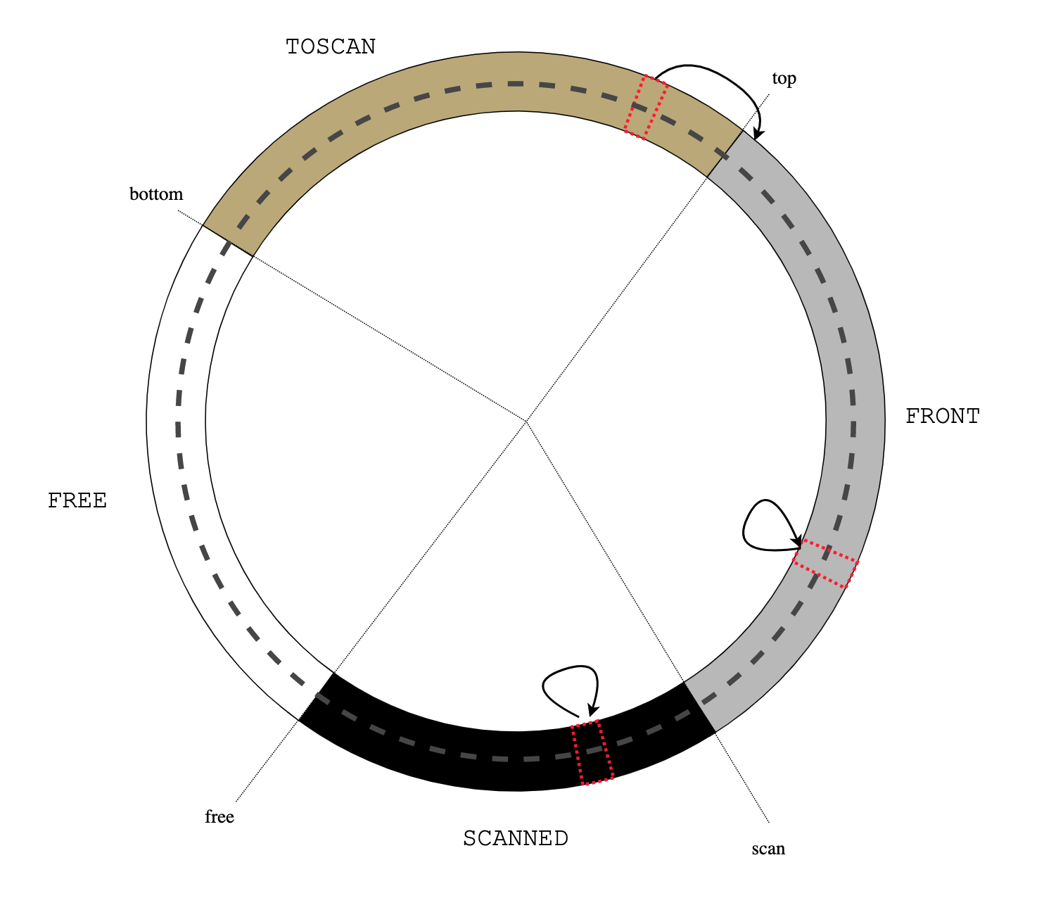
|
| Figure 3: read barrier |
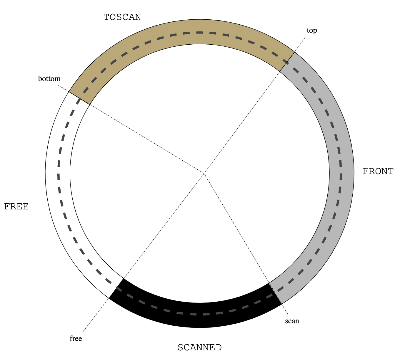
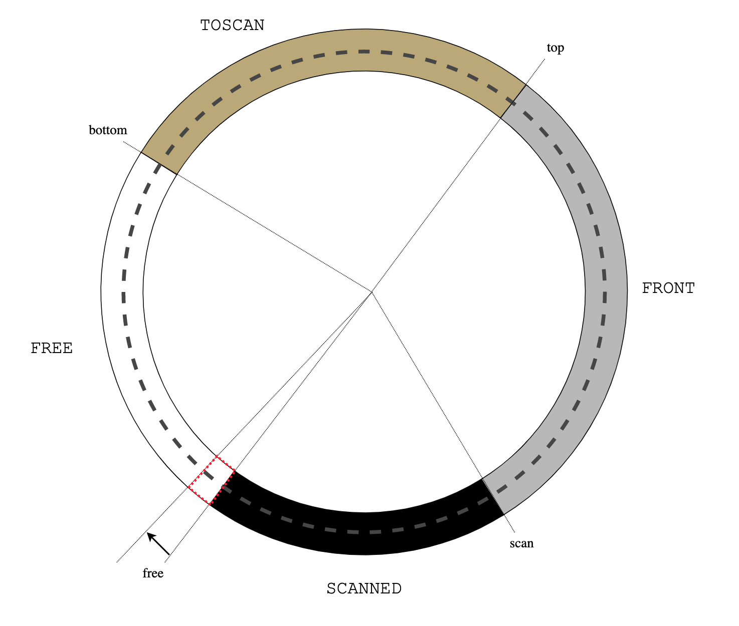
advance() { /* Scan the object pointed to by "scan". */
        for field in pointers(scan) {
                if ecru(scan.field) {
                        darken(scan.field);
                }
        }
        scan := scan.prev; /* Make it black. */
}
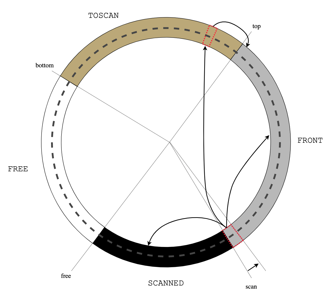 |
| Figure 4: advance() |
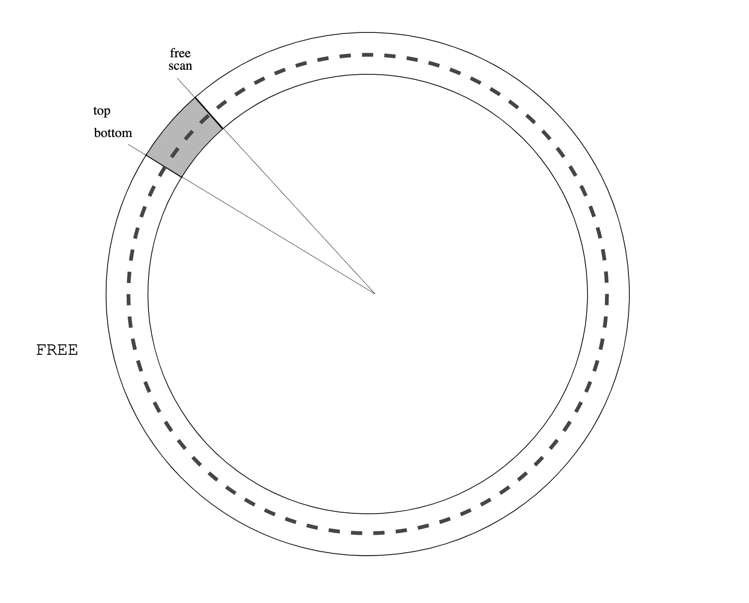
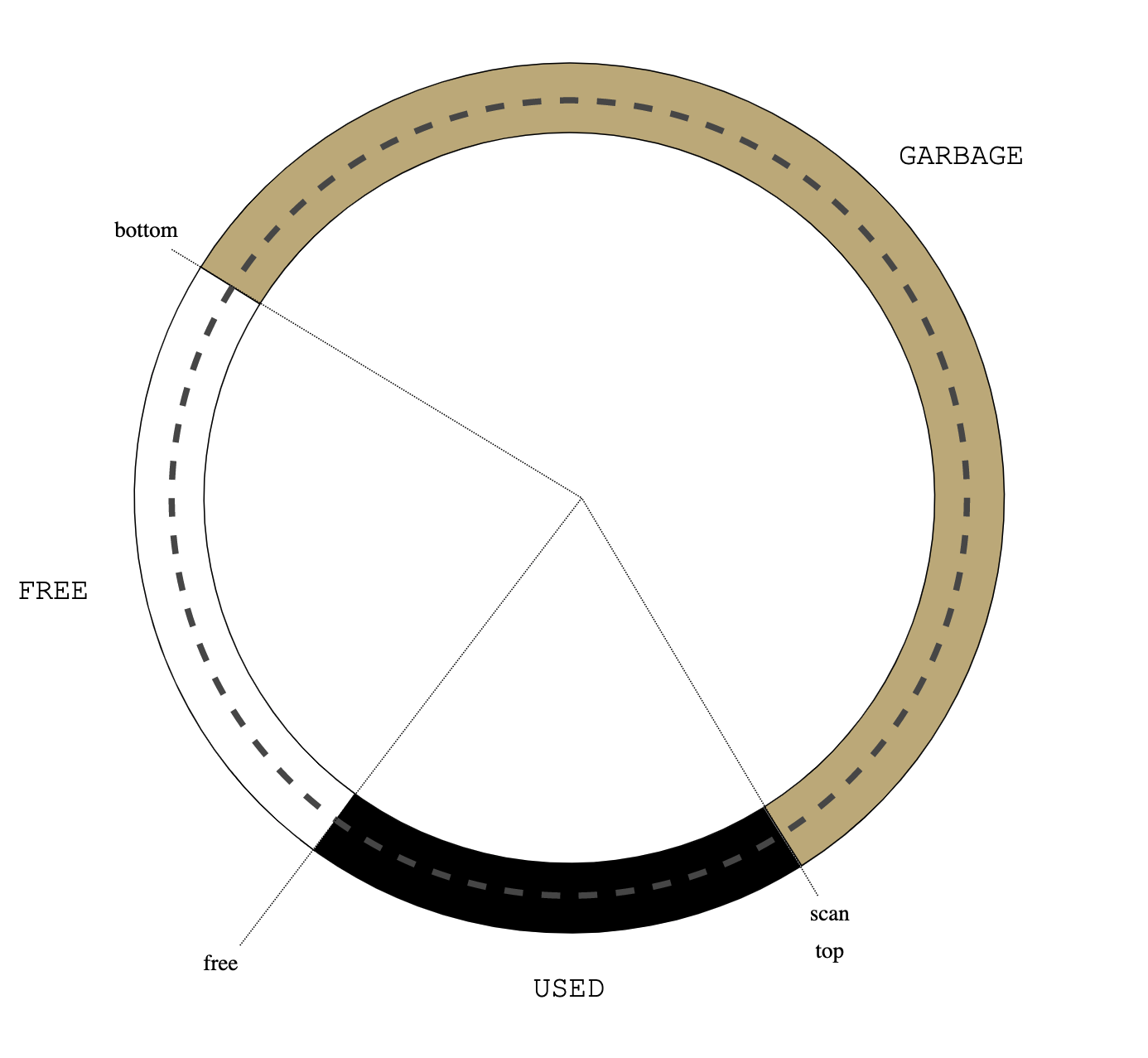 |
| Figure 5: no gray objects |
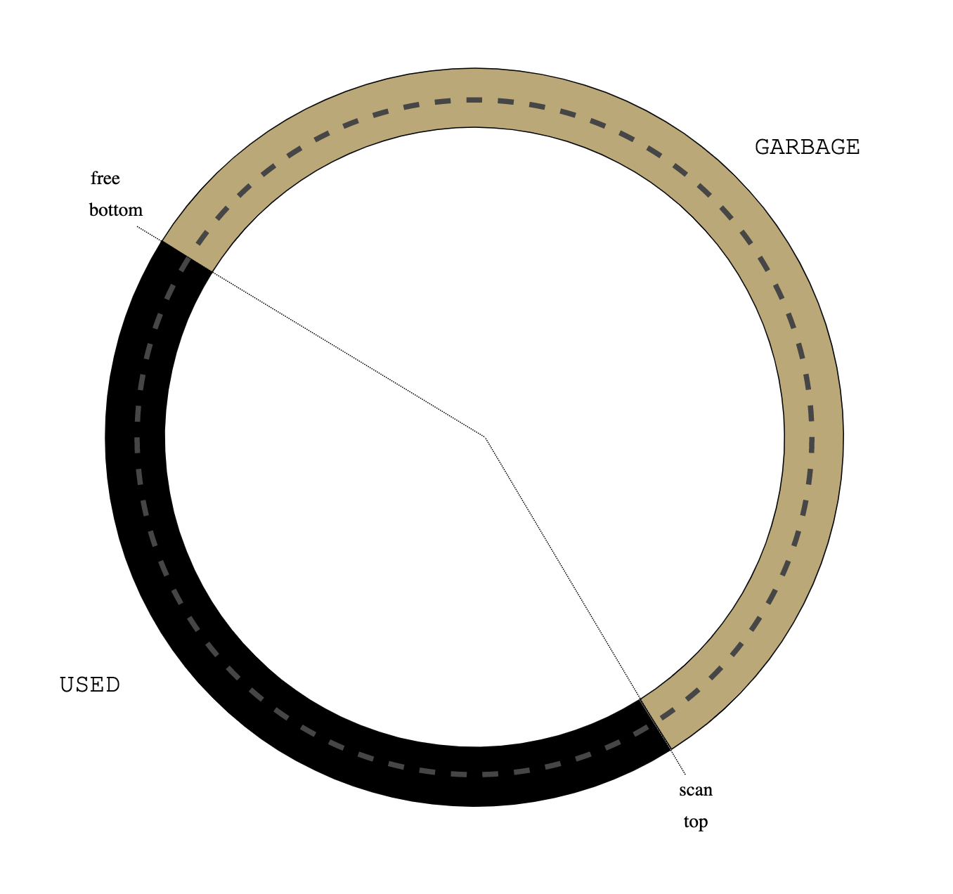 |
| Figure 6: neither gray nor white |
 |
| Figure 7: flip |
 |
| Figure 8: new cycle |


By sheer luck, the first painting is just few kilometers away from me in Pushkin's museum.
a*b + c*d" is converted to "a b * c d * +". An expression in reverse Polish notation can be seen as a program for a stack automaton:
PUSH A
PUSH B
MUL
PUSH C
PUSH D
MUL
ADD
Where PUSH pushes its argument on the top of the (implicit) stack, while ADD and MUL pop 2 top elements from the stack, perform the respective operation and push the result back.
For reasons that will be clearer anon, let's re-write this program as
Container c;
c.put(A);
c.put(B);
c.put(c.get() * c.get())
c.put(C);
c.put(D);
c.put(c.get() * c.get())
c.put(c.get() + c.get())
Where Container is the type of stacks, c.put() pushes the element on the top of the stack and c.get() pops and returns the top of the stack. LIFO discipline of stacks is so widely used (implemented natively on all modern processors, built in programming languages in the form of call-stack) that one never ask whether a different method of evaluating expressions is possible.
Here is a problem: find a way to translate infix notation to a program for a queue automaton, that is, in a program like the one above, but where Container is the type of FIFO queues with c.put() enqueuing an element at the rear of the queue and c.get() dequeuing at the front. This problem was reportedly solved by Jan L.A. van de Snepscheut sometime during spring 1984.
While you are thinking about it, consider the following tree-traversal code (in some abstract imaginary language):
walk(Treenode root) {
        Container todo;
        todo.put(root);
        while (!todo.is_empty()) {
                next = todo.get();
                visit(next);
                for (child in next.children) {
                        todo.put(child);
                }
        }
}
Where node.children is the list of node children suitable for iteration by for loop.
Convince yourself that if Container is the type of stacks, tree-walk is depth-first. And if Container is the type of queues, tree-walk is breadth-first. Then, convince yourself that a depth-first walk of the parse tree of an infix expression produces the expression in Polish notation (unreversed) and its breadth-first walk produces the expression in "queue notation" (that is, the desired program for a queue automaton). Isn't it marvelous that traversing a parse tree with a stack container gives you the program for stack-based execution and traversing the same tree with a queue container gives you the program for queue-based execution?
I feel that there is something deep behind this. A. Stepanov had an intuition (which cost him dearly) that algorithms are defined on algebraic structures. Elegant interconnection between queues and stacks on one hand and tree-walks and automaton programs on the other, tells us that the correspondence between algorithms and structures goes in both directions.
Since Cantor's "I see it, but I cannot believe it" (1877), we know that \(\mathbb{R}^n\) are isomorphic sets for all \(n > 0\). This being as shocking as it is, over time we learn to live with it, because the bijections between continua of different dimensions are extremely discontinuous and we assume that if we limit ourselves to any reasonably well-behaving class of maps the isomorphisms will disappear. Will they?
Theorem. Additive groups \(\mathbb{R}^n\) are isomorphic for all \(n > 0\) (and, therefore, isomorphic to the additive group of the complex numbers).
Proof. Each \(\mathbb{R}^n\) is a vector space over rationals. Assuming axiom of choice, any vector space has a basis. By simple cardinality considerations, the cardinality of a basis of \(\mathbb{R}^n\) over \(\mathbb{Q}\) is the same as cardinality of \(\mathbb{R}^n\). Therefore all \(\mathbb{R}^n\) have the same dimension over \(\mathbb{Q}\), and, therefore, are isomorphic as vector spaces and as additive groups. End of proof.
This means that for any \(n, m > 0\) there are bijections \(f : \mathbb{R}^n \to \mathbb{R}^m\) such that \(f(a + b) = f(a) + f(b)\) and, necessary, \(f(p\cdot a + q\cdot b) = p\cdot f(a) + q\cdot f(b)\) for all rational \(p\) and \(q\).
I feel that this should be highly counter-intuitive for anybody who internalised the Cantor result, or, maybe, especially to such people. The reason is that intuitively there are many more continuous maps than algebraic homomorphisms between the "same" pair of objects. Indeed, the formula defining continuity has the form \(\forall x\forall\epsilon\exists\delta\forall y P(x, \epsilon, \delta, y)\) (a local property), while homomorphisms are defined by \(\forall x\forall y Q(x, y)\) (a stronger global property). Because of this, topological categories have much denser lattices of sub- and quotient-objects than algebraic ones. From this one would expect that as there are no isomorphisms (continuous bijections) between continua of different dimensions, there definitely should be no homomorphisms between them. Yet there they are.
package main
type foo interface {
        f() int
}

type bar struct {
        v int
}


func out(s foo) int {
        return s.f() - 1
}

func (self bar) f() int {
        return self.v + 1
}

func main() {
        for {
                out(bar{})
        }
}
func convT64(val uint64) (x unsafe.Pointer) {
	if val == 0 {
		x = unsafe.Pointer(&zeroVal[0])
	} else {
		x = mallocgc(8, uint64Type, false)
		*(*uint64)(x) = val
	}
	return
}
Abstract: Dual of the familiar construction of the graph of a function is considered. The symmetry between graphs and cographs can be extended to a suprising degree.